Understanding GPU Straggler Ranks and NCCL Basics - p1

25 May, 2026

This blog is written by a human [1]

Say I'm running a distributed ML training job. A total of 4 GPUs in my cluster and one rank mapped to each GPU. I look at the logs for one of the ranks and I see this:

[21:10:49] [rung3-a Rank 0] epoch=0 step=260, loss=4.1811, elapsed=233.3s, dt=8.90s
[21:10:58] [rung3-a Rank 0] epoch=0 step=270, loss=4.3926, elapsed=242.3s, dt=9.00s
[21:11:07] [rung3-a Rank 0] epoch=0 step=280, loss=1.7816, elapsed=251.3s, dt=9.02s
[21:11:16] [rung3-a Rank 0] epoch=0 step=290, loss=2.8534, elapsed=260.3s, dt=8.95s
[21:11:38] [rung3-a Rank 0] epoch=0 step=300, loss=3.0415, elapsed=281.7s, dt=21.46s <- what happened here?
[21:12:26] [rung3-a Rank 0] epoch=0 step=310, loss=4.6558, elapsed=330.3s, dt=48.59s <- what happened here?
[21:13:15] [rung3-a Rank 0] epoch=0 step=320, loss=4.0317, elapsed=378.9s, dt=48.57s <- what happened here?
[21:13:32] [rung3-a Rank 0] epoch=0 step=330, loss=3.2557, elapsed=395.3s, dt=16.47s <- what happened here?
[21:13:40] [rung3-a Rank 0] epoch=0 step=340, loss=3.2556, elapsed=404.3s, dt=8.92s
[21:13:50] [rung3-a Rank 0] epoch=0 step=350, loss=4.5684, elapsed=413.7s, dt=9.43s
[21:13:59] [rung3-a Rank 0] epoch=0 step=360, loss=4.8076, elapsed=422.5s, dt=8.85s
[21:14:08] [rung3-a Rank 0] epoch=0 step=370, loss=5.3923, elapsed=431.5s, dt=8.92s
[21:14:17] [rung3-a Rank 0] epoch=0 step=380, loss=2.5849, elapsed=440.4s, dt=8.96s

You will notice that at some step 300 onwards my $Δ t$ starts ballooning. I check the logs for all my other ranks and I see the exact same thing at the same time. I do have the option of ignoring these logs but then I remember that ML training jobs run for a really really long time. So, purely as a thought experiment, if you assume that a single step is expected to take $Δ t = X$ seconds to run but every 10 steps I see the $Δ t$ goes up by additional $Y$ seconds then on an average I'm taking $(X + \frac{Y}{10})$ per step. In reality this can be much worse. If my model runs for ~300k steps then this occasional latency spike could accumulate and lead to significant additional training time (weeks!).

But do the additional few weeks of training time matter if my model is already training for a few months? The overhead could be justified if your GPUs were doing any actual work during those $Δ t$ spikes but most probably they have already finished their work and are waiting on the "AllReduce" operation to go through.

Glossary

I'm gonna dumb it down to some extent but here is some jargon that you'd care about when working on distributed ML training jobs:

World Size (N) for a training job: The total number of GPU cores that job is training on
Rank: The unique number assigned to the GPU in that world (from 0 to N-1)

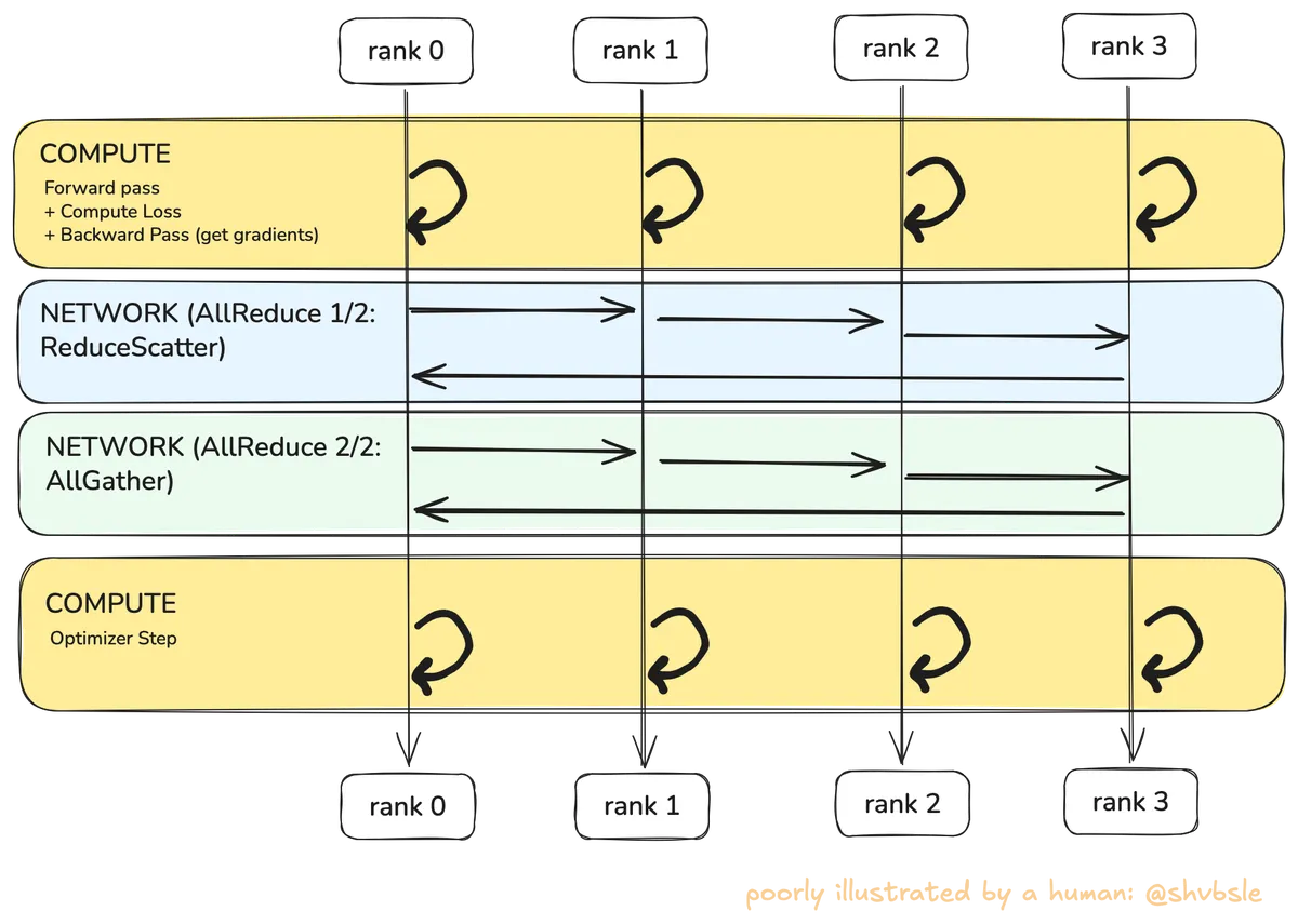
The training step looks like this for each rank:

Each of these N ranks gets a unique "chunk" of data from a large training dataset (Disk I/O)
Forward pass (Compute)
Compute loss (Compute)
Backward pass i.e. generate gradients (Compute)
Synchronize gradients (Network)
Optimizer step (Compute)

To dumb it down further, an ML training job breaks down into three "modes":

Compute: This is the forward-pass, loss, backward-pass, optimization
Network: This is when each rank is exchanging its gradient
Disk I/O: This is reading/writing model weights from disk (or any other operation)

modes of operation: Notice that during compute, nothing leaves the node

Since we'll be talking about NCCL next, here is some additional jargon specifically for NCCL related sections:

NCCL Topology: The topological path (Ring, Tree) over which the AllReduce operation will happen
Ring: NCCL arranges ranks into a ring when passing large volume data for AllReduce. For example chunks flow from rank 0->1->2->3->0. Ring algorithms have a $O (N)$ time complexity in latency but optimal when bandwidth dominates latency. I will speak more on the bandwidth implications in the next sections.
Trees: Another topological arrangement for low latency data transfer (small messages). Trees have $O (l o g N)$ time complexity in latency and useful when latency dominates bandwidth. I will not dive deep into this.
Channels: One channel maps to one instance of the topology that NCCL chooses (could be ring or a tree). Parallelization construct for maximizing network bandwidth.
NCCL Transport: The physical network paths that NCCL uses when moving data between GPUs. Training jobs require moving data between GPUs on the same node and GPUs across nodes. These are some of the popular transports (and there are many more):

Transport	Meaning
`NET/Socket`	TCP over Ethernet (slowest inter-node)
`NET/IB`	InfiniBand/RoCE RDMA (fast inter-node)
`P2P/NVLink`	Direct GPU-GPU via NVLink (intra-node)

Building up intuition for NCCL AllReduce

Now I want to build up some intuition for NCCL AllReduce and where it comes in during an ML training job. A NCCL AllReduce operation is summing the gradients from all ranks and giving that full sum to all ranks. AllReduce is a combination of ReduceScatter and AllGather (note that in the stream I kept referring to ReduceScatter as AllScatter which is incorrect).

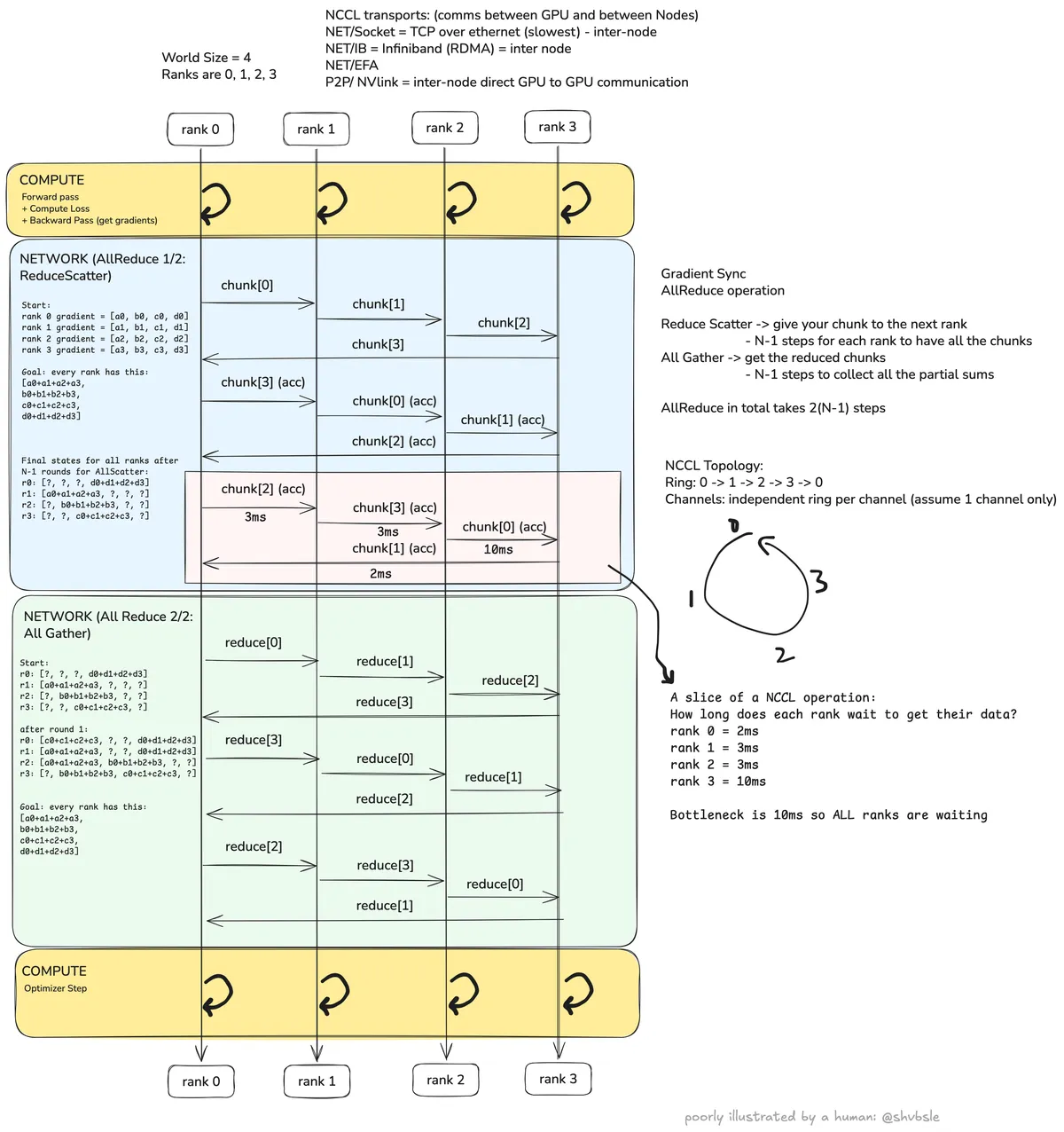
Once every rank does the "compute" step i.e. the yellow block in the diagram it's time to exchange the gradients. I'm going to take some toy data to explain this stage:

Say this is the start state for every rank (each is a vector of four gradient chunks):

Rank 0 gradients: $[a_{0}, b_{0}, c_{0}, d_{0}]$
Rank 1 gradients: $[a_{1}, b_{1}, c_{1}, d_{1}]$
Rank 2 gradients: $[a_{2}, b_{2}, c_{2}, d_{2}]$
Rank 3 gradients: $[a_{3}, b_{3}, c_{3}, d_{3}]$

Then the goal of AllReduce is to get every rank to:

Rank 0 gradients: $[a_{0} + a_{1} + a_{2} + a_{3}, b_{0} + b_{1} + b_{2} + b_{3}, c_{0} + c_{1} + c_{2} + c_{3}, d_{0} + d_{1} + d_{2} + d_{3}]$
Rank 1 gradients: $[a_{0} + a_{1} + a_{2} + a_{3}, b_{0} + b_{1} + b_{2} + b_{3}, c_{0} + c_{1} + c_{2} + c_{3}, d_{0} + d_{1} + d_{2} + d_{3}]$
Rank 2 gradients: $[a_{0} + a_{1} + a_{2} + a_{3}, b_{0} + b_{1} + b_{2} + b_{3}, c_{0} + c_{1} + c_{2} + c_{3}, d_{0} + d_{1} + d_{2} + d_{3}]$
Rank 3 gradients: $[a_{0} + a_{1} + a_{2} + a_{3}, b_{0} + b_{1} + b_{2} + b_{3}, c_{0} + c_{1} + c_{2} + c_{3}, d_{0} + d_{1} + d_{2} + d_{3}]$

`ReduceScatter` and `AllGather`

As shown in the diagram, every rank in the ring will send it's chunk of gradients to the next rank in the ring. We can see from the diagram that it will take $N - 1$ steps for every rank to accumulate one fully-reduced chunk.

So at round 1 we'd have something like these accumulated chunks:

Rank 0 accumulated: $d_{0} + d_{3}$
Rank 1 accumulated: $a_{0} + a_{1}$
Rank 2 accumulated: $b_{1} + b_{2}$
Rank 3 accumulated: $c_{2} + c_{3}$

After $N - 1$ rounds this is what I can construct:

Rank 0 gradients: $[?, ?, ?, d_{0} + d_{1} + d_{2} + d_{3}]$
Rank 1 gradients: $[a_{0} + a_{1} + a_{2} + a_{3}, ?, ?, ?]$
Rank 2 gradients: $[?, b_{0} + b_{1} + b_{2} + b_{3}, ?, ?]$
Rank 3 gradients: $[?, ?, c_{0} + c_{1} + c_{2} + c_{3}, ?]$

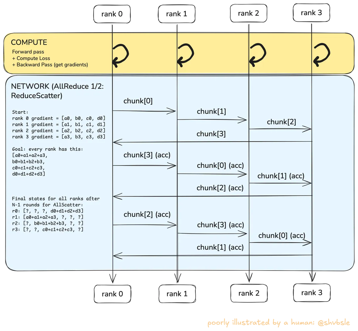
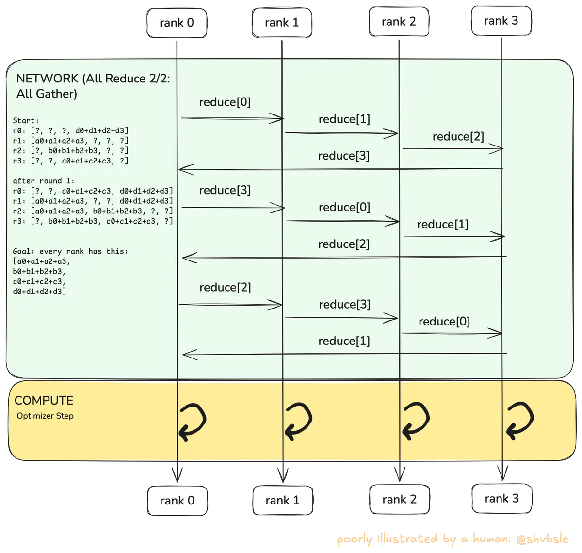
The ? is intentional and I want to show how after N-1 steps, each rank still has 1/4th of all the data that is required to construct the the goal-state we show above. This is where AllGather comes in and does another $N - 1$ trips in the ring to collect the partial reductions.

So the first round of AllGather would look like:

Rank 0 gradients: $[?, ?, c_{0} + c_{1} + c_{2} + c_{3}, d_{0} + d_{1} + d_{2} + d_{3}]$
Rank 1 gradients: $[a_{0} + a_{1} + a_{2} + a_{3}, ?, ?, d_{0} + d_{1} + d_{2} + d_{3}]$
Rank 2 gradients: $[a_{0} + a_{1} + a_{2} + a_{3}, b_{0} + b_{1} + b_{2} + b_{3}, ?, ?]$
Rank 3 gradients: $[?, b_{0} + b_{1} + b_{2} + b_{3}, c_{0} + c_{1} + c_{2} + c_{3}, ?]$

And this continues till we get to the goal i.e. all ranks get:

[a_{0} + a_{1} + a_{2} + a_{3}, b_{0} + b_{1} + b_{2} + b_{3}, c_{0} + c_{1} + c_{2} + c_{3}, d_{0} + d_{1} + d_{2} + d_{3}]

So in effect, AllReduce takes $2 * (N - 1)$ steps. Tree algorithms give you $O (l o g N)$ latency for the same operation, but in a tree all data flows through the root node's link, making it a bottleneck for large messages. In a ring, every link carries an equal share of the total data so no single link is a bottleneck. This is why NCCL uses rings for gradient sync when the model gradients are large (hundreds of MB to GB). You want a bandwidth-optimal algorithm even if it takes more rounds.

Finally, let's talk about the straggler ranks

Let's look at the following diagram: Assume you are in the middle of an ReduceScatter operation. Suppose these are the latencies for data transfer between the ranks:

Rank 0 to Rank 1: 2ms
Rank 1 to Rank 2: 2ms
Rank 2 to Rank 3: 52ms (straggler!)
Rank 3 to Rank 0: 2ms

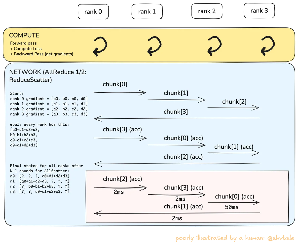
Every step in the ring, i.e. every consecutive rank transfer happens in parallel. To go from step $s$ to $s + 1$ , we have to wait for all ranks to finish their transfers. The bottleneck here is that you are waiting for the slowest rank to finish. So even though Rank 3 sent its reduced chunk to Rank 0 in 2ms, it's still gonna have to wait for 50ms before it moves on to the next step. And hence we see the inflated $Δ t$ across all ranks. This is the straggler rank. Phew!

The problem with stragglers is that they manifest as "inflations" in your training step and do not exactly pin-point which rank causes them and WHY they are caused. Do note that network faults are NOT THE ONLY reason behind rank stragglers. There are many more. I start here because they are easiest to intuit (but still pretty tricky to catch).

We also haven't exactly answered if in this example it was rank 2 at fault or rank 3 i.e. was rank 2 just slow to send out data or rank 3 slow to receive the data? It can be surprisingly hard to answer these questions. In the next-live stream (and next part of this blog) I will explain how to answer these questions. More specifically we will discuss the learnings from this pull-request in k10s that measures network stragglers induced by latency, packet-loss and bandwidth throttle faults.

Improvements:

If you find mistakes or want to suggest improvements to this blog please drop me an email at email with subject: "Blog Improvement" and I'd be happy to credit you for your inputs

Appendix

A. The full illustration from the live-stream:

Footnotes:

Is this AI generated? No it's written by a human. Here is the live-stream as proof (gotta beat those AI-slop allegations I guess lol).

#DDP #GPUs #NCCL #stragglers #training